
When I head out on a journey, whether for vacation or for work, there is always that anticipation along the way. When I finally reach my destination, I get a feeling of accomplishment. I finished something that I started.
If you have been keeping up with the articles on Using Databases with Dispersion Modeling (The Basics, Simple Queries, Calculations With Queries, Calculation Examples, More on Queries, and Nested Queries), I hope to give you that feeling of accomplishment by the end of this article.
Where Did We Begin?
The premise of using a database for dispersion modeling was to more quickly get a result when employing the unitized emission rate dispersion modeling screening technique. When using this technique with a refined dispersion model, e.g. AERMOD, a lot of data is produced for the results. Typically, this problem has been handled with multi-page spreadsheet notebooks. With the ability to produce more data quicker and having more questions to answer with the data, spreadsheets are just not a practical tool anymore.
Databases are designed and optimized to handle huge datasets, like the kind produced when using the unitized emission rate technique. When trying to expedite a modeling analysis and review of that analysis, a database is THE best tool.
Step 1: Build Tables
To use the unitized emission rate modeling technique, you need to build three database tables. These tables can be quickly constructed with SQL statements.
Step 2: Populate Tables
Once you have created your data tables, you will need to populate those tables with your project specific data.
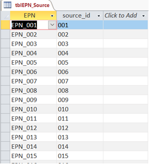
First, populate table tblEPN_Source with the identifiers of the project emission sources, as listed in the project air quality permit application or in the current version of the air quality permit, with the associated source identifier used in the dispersion model input. Your table should like something like this:
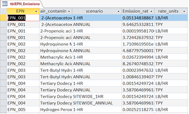
Next, populate table tblEPN_Emissions with the identifiers of the project emission sources, air contaminant name, emission rate to be modeled, and the units of the emission rate. Typically, the units will be pounds per hour (LB/HR) or tons per year (TPY). Your table should like something like this:
Step 3: Import Your Model Results
When using the unitized emission rate modeling technique, the model (AERMOD), will generate a rather large result file, on the order of 10-100 MB. Not huge, but definitely large. The next step is to import the data from the AERMOD PLOTFILE that contain a listing of all the unitized concentrations.
The import process consists of three steps: Reformat, Import, and Insert.
To start the import process with the raw PLOTFILE, you will need to have the data reformatted so it is in a more recognizable format to the database platform. To achieve this, we have a utility (NKAermodToCSV.exe) that reformats either PLOTFILEs or MAXIFILEs to a comma separated value (CSV) text file. In addition, a field is created in the file, “FILE_NAME”, that contains the name of the file being reformatted. This utility is not ready for prime-time, but we can email it to you upon request ([email protected]).
Once the data are reformatted, the newly recreated file can be imported into a database platform. For our example we have used an Access database.
This video shows the reformatting tool in action.
Once your model results are in your database, the next step is to insert the model results data into another data table. The reason for the two step process is the raw data is coming from a data source external to the database you are using. There is always a chance that bad data could be in the raw data, so the import process will catch any invalid entries. By isolating the imported data from the rest of the database, you can focus on fixing the raw data while keeping the rest of data tables and associated queries untouched.
After you have finished your QA/QC of the imported data, you can insert the modeling results into the table tblAERMOD_PLOTFILE.
Step 4: Build Queries for Results
When all of your data (sources, emission rates, and model results) has populated your database tables, you will need to query these data to produce a summary of the modeling results.
The pseudo-code for a query to return the maximum predicted concentration for each air contaminant in your analysis would look something like:
SELECT
    MAX(SUM((unitized concentrations)*(air contaminant emission rate)))
        for each air contaminant
FROM
    (SELECT
        SUM((unitized concentrations)*(air contaminant emission rate))
            for each air contaminant at each receptor
    FROM
        (SELECT
            (unitized concentrations)*(air contaminant emission rate)
            for each source and each air contaminant at each receptor
        FROM
        (PLOTFILE results table)))
In red, you are multiplying the unitized concentration by the emission rate (products) for each source, each air contaminant, at each receptor.
In blue, you are summing all the products (sum of the products) for each air contaminant at each receptor.
Finally, in black, you take the maximum of the sum of the products for each air contaminant.
The complete SQL statement to perform all the necessary calculations can be found at SOP Document.
Step 5: Execute Queries
All the pieces are together. You have the data and the means to access, manipulate, and analyze the data. See the video below to see how little time it takes to get results summarizing over 100 sources and nearly a 100 air contaminants at over 10,000 receptors.
The actual run time for the queries was about 10 minutes without indexes added to the tables. Once indexes were added the run time was about 3 minutes. If you decide to build your database in SQL server, the query run time will be mere seconds.
Summary
So now we have reached a point where we have put all the pieces together to perform a set of tasks in a few minutes that used to typically take hours. By using the right tool with your project, time and effort. The database is the right tool for storing, manipulating, and analyzing model results.
You have seen how to build the database, fill the database, and use the database. Now it is time to put what you have learned into action. Use a database on your next project. I almost guarantee you will never go back to using spreadsheets again.
If you found this article informative, there is more helpful and actionable information for you. Go to http://learn.naviknow.com to see a list of past webinar mini-courses. Every Wednesday (Webinar Wednesday), NaviKnow is offering FREE webinar mini-courses on topics related to air quality dispersion modeling and air quality permitting. If you want to be on our email list, drop me a line at [email protected].
One of the goals of NaviKnow is to create an air quality professional community to share ideas and helpful hints like those covered in this article. So if you found this article helpful, please share with a colleague.